1. Prediction of fluid velocity distribution from pore structure in porous media (MIT, UT-Austin)
Research thrusts: Fast & reliable solution of multiphysics/multiscale problems
Research sub-thrusts: Fast solvers; Accurate & robust discretizations; Coarse graining
Porous media flows have a rich structure, and this spatial and temporal complexity plays a critical role in natural and engineered processes such as groundwater contamination and remediation, water infiltration in soil, geologic carbon sequestration, enhanced hydrocarbon recovery, water filtration systems, and polymer electrolyte fuel cells. Understanding and quantifying velocity heterogeneity in porous media is important because it controls particle spreading and fluid mixing, which often mediates chemical reactions and biological activity. The groups of co-PI Juanes at MIT and co-PI Biros at UT Austin have been collaborating to address a long-standing challenge in porous media flows: predicting the relationship between pore structure and velocity distribution from Stokesian flow through the pore space [42]. We derive an analytical relationship between the pore throat size distribution fλ ~ λ-β and the distribution of fluid velocity fu ~ u-β∕2, based on a conceptual model of porelets—Hagen–Poiseuille flows established within each pore throat. Our model allows us to make predictions for the statistics of spreading of fluid particles along their own trajectories, which are confirmed by high fidelity simulations of Stokes flow and advective transport (Fig. 1). The proposed theoretical framework can be extended to other configurations that can be represented as a collection of known flow distributions. Ongoing work seeks to extend the framework to more complex media.
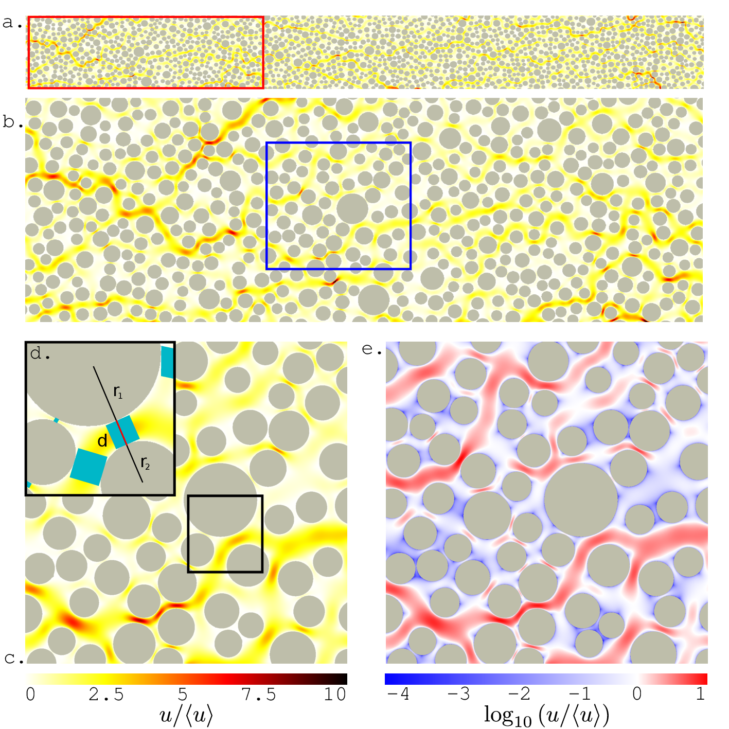
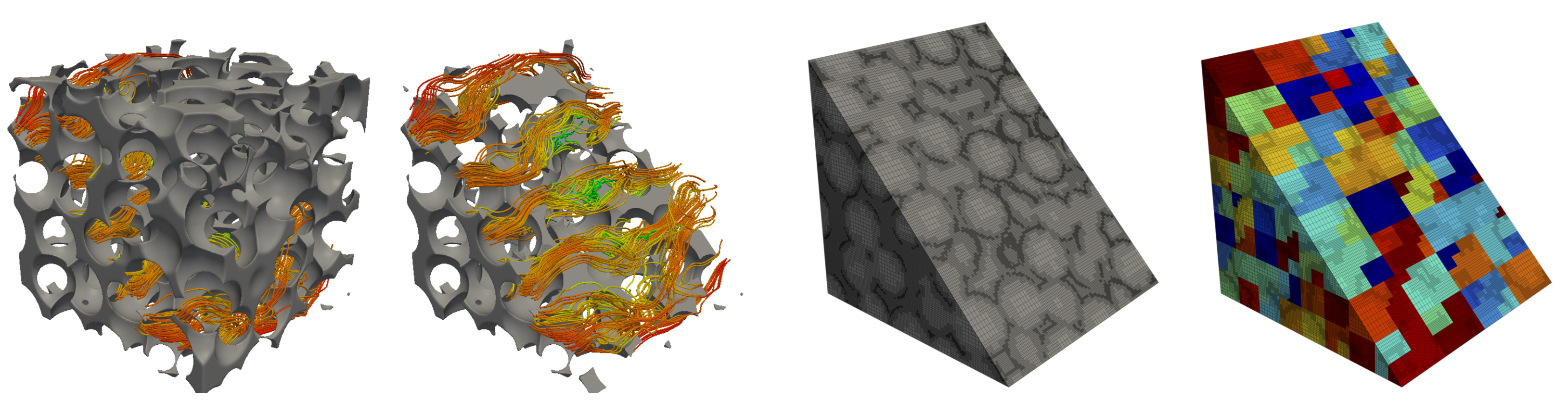
As we can see in Fig. 1 the Stokes flow is resolved to very high resolution. Accurate direct numerical simulation of Stokes flow in the pore scale is itself extremely challenging due to the complex pore microstructure, the indefinite elliptic operators, and complex geometries. In two dimensions, boundary integral equations can be used. But in 3D and for geometries that have random structure, boundary integrals become much more challenging. To address this, we developed a novel numerical scheme for solving the Stokes equation with variable coefficients in the unit box. Our scheme is based on a volume integral equation formulation. Compared to finite element methods, our formulation decouples the velocity and pressure and generates velocity fields that are by construction divergence free to high accuracy, and its performance does not depend on the order of the basis used for discretization. In addition, we employ a novel adaptive fast multipole method for volume integrals to obtain a scheme that is algorithmically optimal and supports non-uniform discretizations. To increase per-node performance, we have integrated our code with both NVIDIA and Intel accelerators. In our largest scalability test, we solved a problem with 20 billion unknowns, using a 14th-order approximation for the velocity, on 2048 nodes of the Stampede system at the Texas Advanced Computing Center. We achieved 0.656 petaFLOPS for the overall code (23% efficiency) and one petaFLOPS for the volume integrals (33% efficiency). This work was a finalist for Best Student Paper at SC14 [89]. Illustrative simulations are shown in Fig. 2.
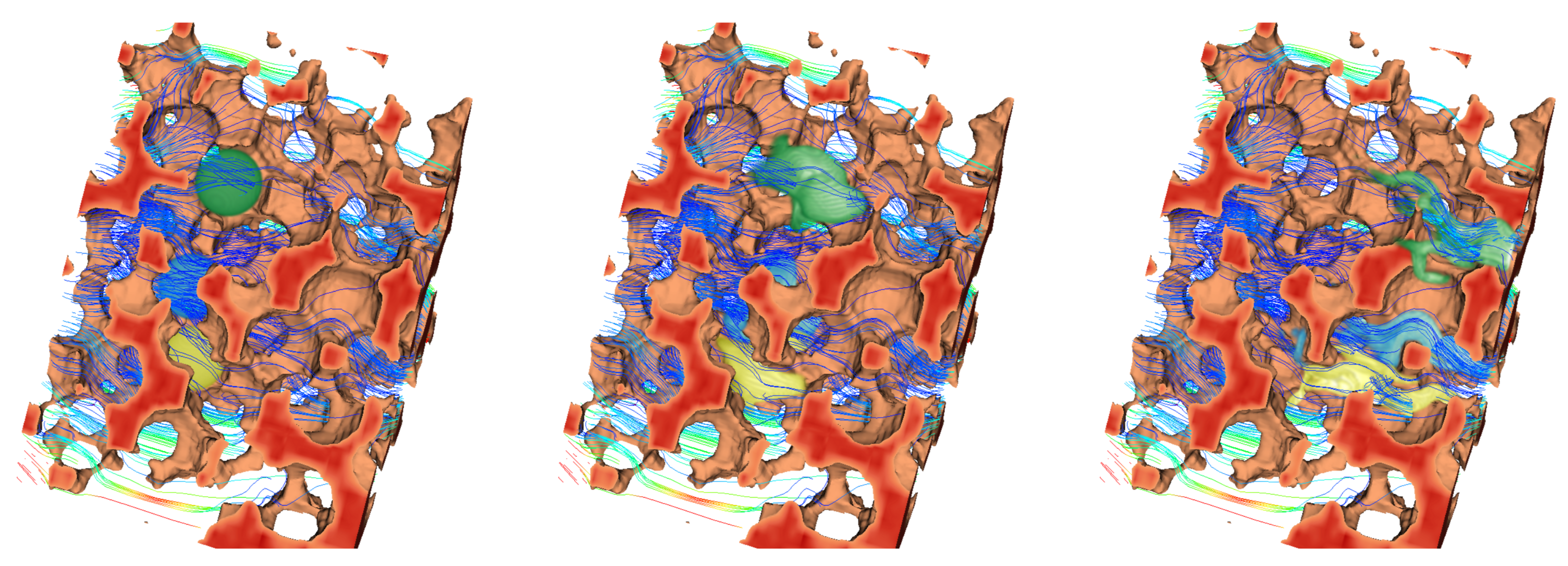
To study transport phenomena in porous media we also need an advection-diffusion solver (Fig. 3). We have designed a novel numerical method for solving the scalar advection-diffusion equation using adaptive mesh refinement. Our solver has three unique characteristics: (1) it supports arbitrary-order accuracy in space; (2) it allows different discretizations for the velocity and scalar advected quantity; (3) it combines the method of characteristics with our volume integral equation formulation; and (4) it supports shared and distributed memory architectures. In particular, our solver is based on a second-order accurate, unconditionally stable, semi-Lagrangian scheme combined with a spatially-adaptive Chebyshev octree for discretization. We have studied the convergence, single-node performance, strong scaling, and weak scaling of our scheme for several challenging flows that cannot be resolved efficiently without using high-order accurate discretizations. For example, we consider problems for which switching from 4th order to 14th order approximation results in two orders of magnitude speedups for a computation in which we keep the target accuracy in the solution fixed. For our largest run, we solve a problem with one billion unknowns on a tree with maximum depth equal to 10 and using 14th-order elements on 16,384 x86 cores on the Stampede system at TACC. This work will appear at SC16 [10].